Ensemble Projection for Semi-supervised Image Classification
Dengxin Dai and Luc Van Gool
Please see the recent results of Ensemble Projection with the CNN features here if you are interested.
Abstract
This paper investigates the problem of semi-supervised
classification. Unlike previous methods to regularize classifying boundaries with unlabeled data, our method learns
a new image representation from all available data (labeled
and unlabeled) and performs plain supervised learning with
the new feature. In particular, an ensemble of image prototype sets are sampled automatically from the available
data, to represent a rich set of visual categories/attributes.
Discriminative functions are then learned on these prototype sets, and image are represented by the concatenation
of their projected values onto the prototypes (similarities
to them) for further classification. Experiments on four
standard datasets show three interesting phenomena: (1)
our method consistently outperforms previous methods for
semi-supervised image classification; (2) our method lets itself combine well with these methods; and (3) our method
works well for self-taught image classification where unlabeled data are not coming from the same distribution as labeled ones,
but rather from a random collection of images.
Overview
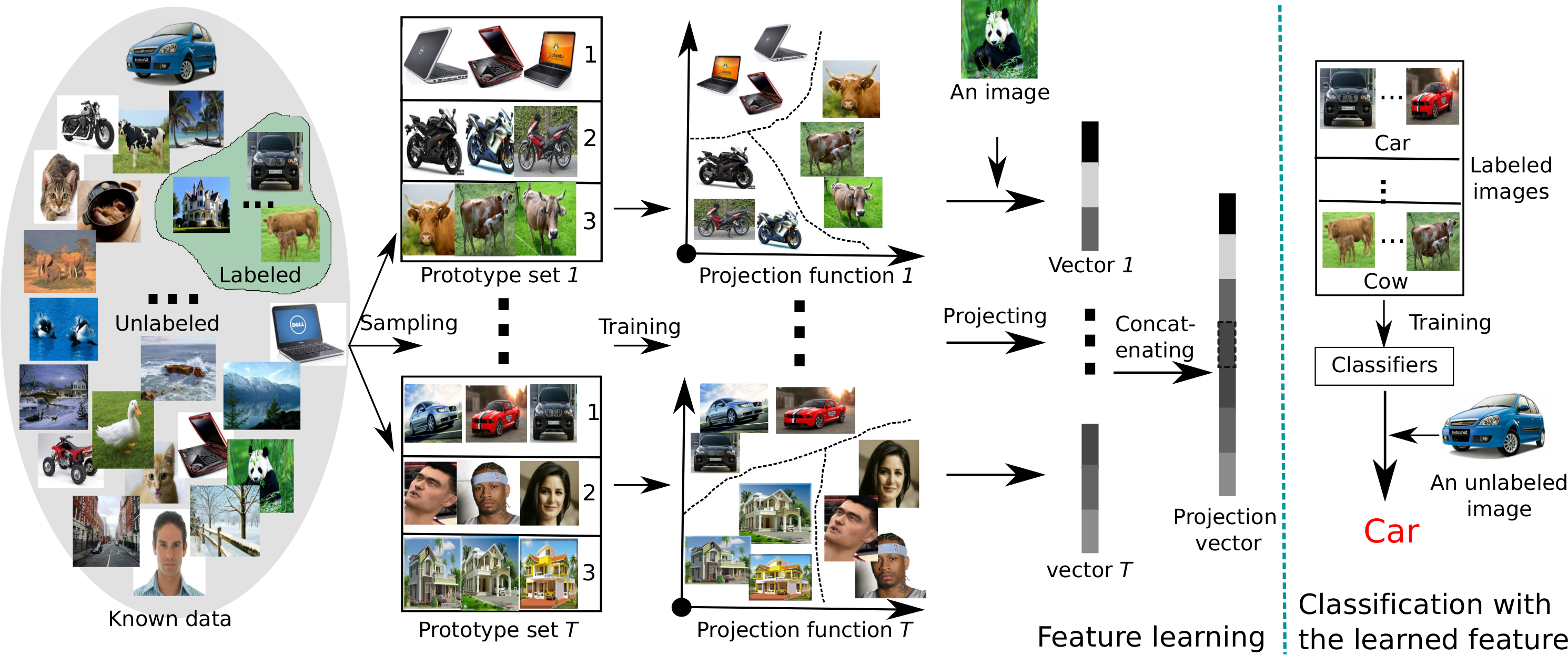
Fig1. The pipeline of Ensemble Projection (EP).
EP consists in unsupervised feature learning (left panel) and plain supervised classification (right panel).
For feature learning, we sample an ensemble of T diverse prototype sets from all known images and learn discriminative
classifiers on them for the projection functions. Images are then projected using these functions to obtain their new representation. For
classification, we train plain classifiers on labeled images with the learned features to classify the unlabeled ones.
Results
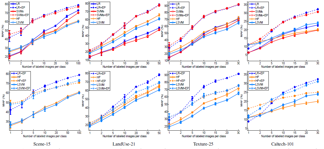
Fig2. Semi-supervised classification results (average ap) on the four datasets. The top panel evaluate the performance of our learned features when
fed into Logistic Regression and SVMs. The bottom shows its performance when fed into HF [34] and LapSVM [1]. All methods were tested with two
feature inputs: the concatenation of GIST, PHOG and LBP, and our learned feature from them (indicated by “+ EP”).
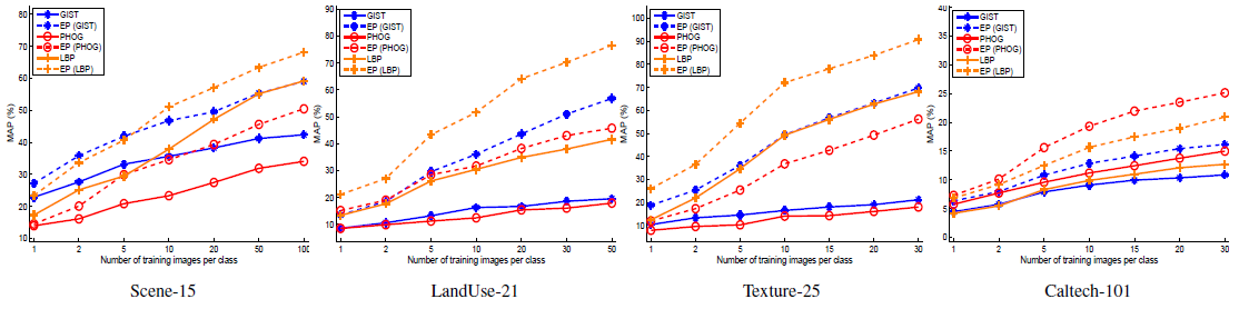
Fig3. Comparison of our learned features (indicated by EP(.)) to the corresponding original features GIST, PHOG, and LBP.
Logistic Regression was used as the classifier with 5 labeled training images per class.
Downloads
Code
The matlab
code of ensemble projection and the
code I used to extract all the features are available to use.
Data
The datasets Scene-15, LandUse-21, Texture-25, and Caltech-101 were used in the paper, with three common image features GIST, PHOG, and LBP.
The features were L1-normalized and then multiplied by their dimensions (e.g. for GIST, the L1-normalized feature values are then multiplied by 20.).
This is to map all feature values to comparable levels.
The data (MAT-File) we used for the paper are:
15_gist,
15_phog,
15_lbp,
21_gist,
21_phog,
21_lbp,
25_gist,
25_phog,
25_lbp,
101_gist,
101_phog,
101_lbp.
Paper
D. Dai and L. Van Gool.
Ensemble Projection for Semi-supervised Image Classification.
ICCV,
2013.
PDF BibTex
Poster
The
Poster presented in ICCV 2013.
This page has been edited by
Dengxin Dai